7.1. Why Not Linear Regression?¶

At this point, a natural question might be why one cannot use linear regression to model categorical outcomes. To understand why, let’s look at an example. We have a data set related to a telephone marketing campaign of a Portuguese banking institution. Suppose we would like to model the likelihood that a phone call recipient will make a term deposit at the bank. The data is saved in a data frame called deposit, and the first few observations are shown below:

head(deposit)

age	marital	education	default	housing	loan	contact	duration	campaign	previous	poutcome
30	married	primary	no	no	no	cellular	79	1	0	unknown
33	married	secondary	no	yes	yes	cellular	220	1	4	failure
35	single	tertiary	no	yes	no	cellular	185	1	1	failure
30	married	tertiary	no	yes	yes	unknown	199	4	0	unknown
59	married	secondary	no	yes	no	unknown	226	1	0	unknown
35	single	tertiary	no	no	no	cellular	141	2	3	failure

These variables are defined as follows:

age: The age of the person contacted.
marital: The marital status of the person contacted.
education: The education level of the person contacted.
default: Whether the person contacted has credit in default.
housing: Whether the person contacted has a housing loan.
loan: Whether the person contacted has a personal loan.
contact: How the person was contacted (cellular or telephone).
duration: The duration of the contact, in seconds.
campaign: The number of contacts performed during this campaign for this client.
previous: The number of contacts performed before this campaign for this client.
poutcome: The outcome of the previous marketing campaign (failure, nonexistent, or success).
subscription: Whether the person contacted made a term deposit (1 if the person made a deposit and 0 if not).

Let’s try using linear regression to model subscription as a function of duration:

depositLinear <- lm(subscription ~ duration, data = deposit)
summary(depositLinear)

Call:
lm(formula = subscription ~ duration, data = deposit)

Residuals:
     Min       1Q   Median       3Q      Max 
-1.47629 -0.11329 -0.05758 -0.01963  1.00009 

Coefficients:
              Estimate Std. Error t value Pr(>|t|)    
(Intercept) -1.488e-02  6.203e-03  -2.399   0.0165 *  
duration     4.930e-04  1.675e-05  29.436   <2e-16 ***
---
Signif. codes:  0 '***' 0.001 '**' 0.01 '*' 0.05 '.' 0.1 ' ' 1

Residual standard error: 0.2926 on 4519 degrees of freedom
Multiple R-squared:  0.1609,	Adjusted R-squared:  0.1607 
F-statistic: 866.5 on 1 and 4519 DF,  p-value: < 2.2e-16

Based on this output, our estimated regression equation is:

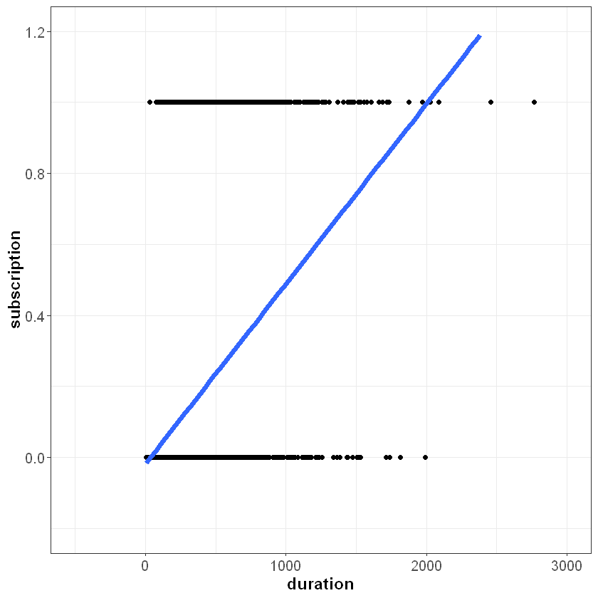
\[predicted \;subscription = \hat{y} = -0.01488 + 0.0004930(duration)\]

If we plot this line on top of our data, we can start to see the problem:

Our independent variable subscription can only take on two possible values, 0 and 1. However, the line we fit is not bounded between zero and one. If duration equals 2,500 seconds, for example, the model would predict a value greater than one:

\[\begin{split}\begin{aligned}predicted \;subscription = \hat{y} & \approx -0.01488 + 0.0004930(2500) \\ & \approx -0.01488 + 1.2325 \\ & \approx 1.2176\end{aligned}\end{split}\]

A negative value of duration does not make sense in this context, but in principle the same problem applies in the opposite direction - for small values of \(X\), the linear model might predict outcomes less than zero. To overcome this issue, logistic regression models the dependent variable \(Y\) according to the logistic function, which is bounded between zero and one.

Data Science for Managers

7.1. Why Not Linear Regression?¶